Sounds 2
Continuous to Categorical
The neural representations of speech that we’ve seen so far in either the temporal envelope tracking or the tone sweep frequency mapping in the STG are all “continuous” representations. That means that there is gradience in the actual neural activity on the cortex, i.e., there’s lots of shades of grey.
But speech perception is ultimately a categorical phenomenon. If I ask 10 of you to say “pa” you will each have 10 different VOTs for the “p” but we will all perceive the utterance as a singular “pa”, that is, there is one category of “p” that our brains represent. The question now becomes, how does the brain move from a continuous representation to a categorical.
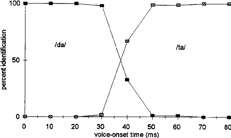
In the image above, imagine you’re listening to a t/d-like syllable, with a particular VOT. Low VOTs are “categorically” identified as “da”, notice that even though the VOT changes by 10ms increments, they’re still all labeled as “da.” Once the VOT gets longer than 30ms, however, we start identifying the sound as “ta”, with a “crossover” at roughly 40ms. This is categorical identification. The stimuli are either da or ta, nothing in between! Our perceptual system (ultimately our brain) imposes this structure on the “continuous” acoustic signal. In the Mesgarani and Chang paper it turns out that the individual electrodes respond in a binary way with respect to features.
Ganong effect
It turns out that our perceptual system which categorically imposes structure on the continuous acoustic signal is affected in a top-down fashion by the lexicon of the language. A famous example of this is the Ganong effect. In the example above, imaging that instead of hearing “da” and “ta”, you’re hearing “d/t-eed”. So on the left end, the stimulus with the smallest VOT is “deed” and the right end the stimulus with the longest VOT is “teed”. It turns out, that that middle stimulus with a VOT of 40ms (which is ambiguously either “d” or “t”) is labelled more as “d” in this case. Why? Because it makes a real word in English, whereas “teed” is not a real word. So in this way, the lexicon is affecting the low-level perception!
Phonemic receptive fields
Again, the question is what neural representation in the brain allows this sort of behaviour to happen? Mesgarani et al. (2014) did a study, again with patitents with electrodes implanted directly in the superior portion of the temporal lobe (this would capture STG, primary auditory cortex).[See the presentation and last lecture tab] Subjects listened to sentences that included a variety of English phonemes. They found that electrodes recorded activity in an “all or nothing” fashion according to phonological features, and these features were spatially distributed in the auditory cortex. So, there would be a different pattern of activation for “d” vs. “t”, which would similar place of articulation activity, but differing voicing activity. In this way, the brain is representing these sounds phonemically.
The brain’s sampling rate
The time scale of the chunks that the brain uses to process information is also important for our understanding of the transformation from continuous acoustic representation to phoneme-like representation. There is evidence that the sampling rate (or how fast the brain takes snapshots of the incoming signal) is at two times: fast (25-40ms) and less fast (200-300ms). Evidence for this comes from a neat (old) experiment [see presentation] by Saberi and Perrorr (1999). Different sections of continuous speech were reversed, but the windows of reversed speech were different lengths, from 300-20ms. Remember, these are pretty fast, with 20ms being the quickest (the length of an average CV is around 500ms). When the reversed segments of speech were very short (30-50ms), participants were 100% accurate–it’s as if nothing happened to the speech! This leads researchers to believe that the sampling rate (or the snapshots) of the brain is on the order of around 30ms, which captures the spectral properties of speech. Another window at around 300ms captures the syllable.